[시계열 분석] ARIMA 모델 | 파이썬 예제

 

ARIMA를 다룬 유튜브 강의와 다양한 기술 블로그들을 참고하여

ARIMA 모델에 대해 간단히 정리해보았고

간단한 파이썬 예제로 코드도 다뤄보려 한다.

---

 

ARIMA 모델은

Autoregressive Integrated Moving Average 라는 뜻으로, 

AR(Autoregression) 모형과 MA(Moving Average) 모형을 합친 모형이다.

 

독립변수과 종속변수를 활용하는 다른 머신러닝 모델과는 달리 시간을 독립변수로 종속변수를 예측한다.

또한, 전통적인 통계 기법을 활용한 모델이기 때문에 통계적인 이해가 어느정도 필요하다.

 

 

0. 정상성

시계열 분석은 데이터가 정상성을 띠어야 한다

시간에 관계없이 평균과 분산이 일정한 시계열 데이터를 정상적이라고 한다.

시간의 흐름에 데이터가 영향을 받는다면, 예로 추세나 계절성이 있다면 그것은 정상 시계열이 아니다.

 

 

비정상적인 데이터는 예측이 제대로 되지 않기 때문에 데이터를 변환시켜야 한다.

• 로그

(b) 그래프는 (a) 그래프를 로그 변환한 것이다.

로그 변환은 좀 더 단순화된 일정한 분산을 갖게 해준다

• 차분

현재 상태에서 이전 상태를 빼주는 것을 의미한다. (Yt - Yt-1) 

(c) 그래프는 (a) 그래프를 차분한 것이다.

차분은 0을 중심으로 평균이 일정하게 유지되는 패턴으로 변환시켜준다.

 

 

 

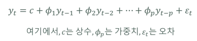
1. AR 모델

특정 변수의 과거 관측값의 선형결합으로 해당 변수의 미래값을 예측하는 모형이다.

과거 p개의 관측값의 선형결합으로 예측하는 모델을 p차 MA모델 (AR(p))라고 표현한다.

 

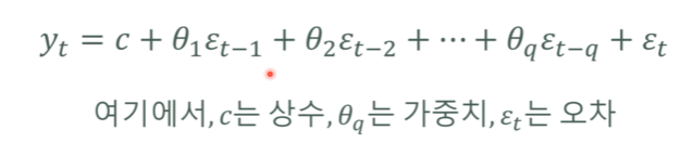
2. MA 모델

예측오차를 이용하여 미래의 값을 예측하는 모형이다.

과거 q개 예측오차의 선형결합으로 예측하는 모델을 q차 MA모델 (MA(q))라고 표현한다.

 

3. ARMA 모델

ARMA모델은 AR모델과 MA모델을 결합한 모델로 ARMA(p,q)로 표현한다.

 

 

4. ARIMA 모델

ARIMA(p,d,q) 모델은 ARMA모델에 차분 과정을 추가한 것이다.

시계열 데이터를 d회 차분하고 과거 p개의 관측값과 q개 오차에 의해 예측되는 모델이다.

 

 

---

 

최적의 p와 q는 ACF와 PACF 그래프를 통해 확인할 수 있다.

 

 

1. ACF(자기상관함수, AutoCorrelation Function)

자기상관은 다른 시점의 관측값 간 상호연관성을 나타낸다.

시차를 적용한 시계열 데이터 간의 상관관계를 의미한다.

ACF 구하는 식, 일반 Correlation 구하는 식과 동일하다

 

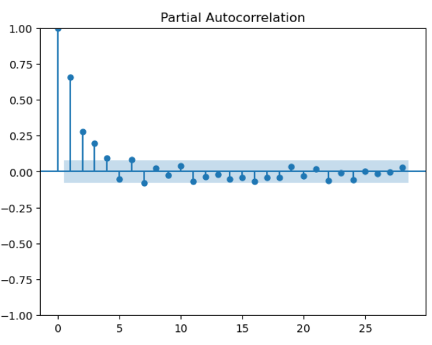
2. PACF(편자기상관함수, Partial AutoCorrelation Function)

편자기상관은 시차가 다른 두 시계열 데이터 간의 순수한 상호 연관성을 나타낸다.

PACk는 원래의 시계열 데이터(Yt)와 시차 k 시계열 데이터(Yt-k)간의 순수한 상관관계로서 두 시점 사이에 포함된 시계열 데이터(Yt-1, Yt-2, ... , Yt-k+1)의 영향은 제거된다.

 

 

acf값이 서서히 줄어들고 있는 모습으로 데이터 간 자기상관이 높다. 즉, 정상적이지 않다.

 

pacf값은 시차 4에서부터 절단면 (신뢰구간 95%) 안에 들어간다.

 

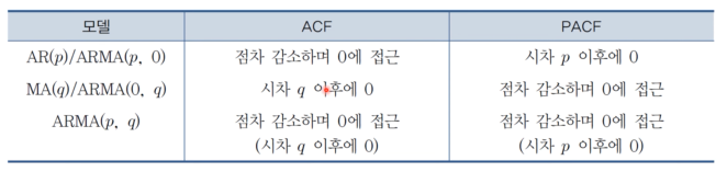
ACF 도표에서 파란색 음영 안에 들어오는 시차(절단점) - 1을 q로 설정한다.

PACF 도표에서 파란색 음영 안에 들어오는 시차(절단점) - 1을 p로 설정한다.

---

 

파이썬 예제

 

# 라이브러리 가져오기

import pandas as pd
import numpy as np
import seaborn as sns
import matplotlib.pyplot as plt

from statsmodels.tsa.stattools import adfuller # ADF 검정
from statsmodels.graphics.tsaplots import plot_acf, plot_pacf # ACF, PACF 그래프
from statsmodels.tsa.arima.model import ARIMA # ARIMA 모델

from sklearn.metrics import mean_absolute_error, mean_squared_error
import math
import itertools

import warnings
warnings.filterwarnings('ignore')

 

df = pd.read_csv("Aquifer_Petrignano.csv")

df.Depth_to_Groundwater = df.Depth_to_Groundwater.interpolate()
df.Depth_to_Groundwater.plot()

 

 

예측하고자 하는 Depth_to_Groundwater 변수 시각화하여 데이터 분포 확인

 

# Date를 7일 간격으로 재조정
df_downsampled = df[['Date', 'Depth_to_Groundwater']].resample('7D', on = 'Date').mean()
df = df_downsampled.reset_index()

plt.figure(figsize = (15,8))

# 1년 = 52주
rolling_window = 52

sns.lineplot(x = df.Date, y = df.Depth_to_Groundwater, color = 'indianred')
sns.lineplot(x = df.Date, y = df.Depth_to_Groundwater.rolling(rolling_window).mean(), color = 'black', label = 'rolling mean') 
sns.lineplot(x = df.Date, y = df.Depth_to_Groundwater.rolling(rolling_window).std(), color = 'blue', label = 'rolling std')
plt.xlim([date(2009,1,1), date(2020,6,30)])
plt.title('Feature : Depth_to_Groundwater', fontsize = 14)
plt.ylabel(ylabel = 'Depth_to_Groundwater', fontsize = 14)
plt.show()

주 단위의 데이터로 1년에 대한 이동평균과 표준편차를 시각화하였다.

 

plt.figure(figsize = (15,7))
sns.distplot(df.Depth_to_Groundwater,  color = 'indianred')
plt.title('Histogram : Depth_to_Groundwater', fontsize = 14)
plt.ylabel(ylabel = 'Depth_to_Groundwater', fontsize = 14);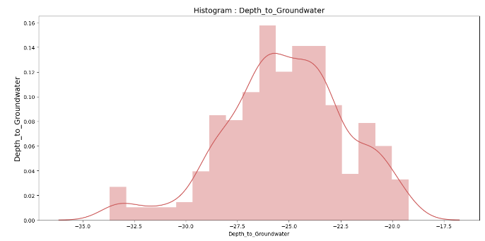

 

정상성 시계열 데이터는 평균, 분산이 가우시안 분포를 따른다.

그래프를 보면 평균과 분산이 어느정도 종 모양을 그리는 것 같다.

 

데이터가 정상서을 따르는지 검증하기 위한 방법이 있는데 이를 ADF 검정이라고 부른다.

 

간단하게 ADF 검정 결과의 p-value 가 0.05 이하이면, 단위근이 없다는 귀무가설을 기각하므로 시계열 데이터가 정상적이지 않다고 추론할 수 있다.

 

result = adfuller(df.Depth_to_Groundwater.values)

print(f'adf_stat : {result[0] : 0.3f}')
print(f'p_val : {result[1] : 0.3f}')
print(f'crit_val_1 : %0.3f' % result[4]['1%'])
print(f'crit_val_1 : %0.3f' % result[4]['5%'])
print(f'crit_val_1 : %0.3f' % result[4]['10%'])

ADF 검정 결과 p value가 0.05보다 낮지만 시각화 그래프를 보면 데이터가 정상적이지 않은 모습을 보이기 때문에 데이터 변환을 거쳐준다.

 

# 로그 변환

df['Depth_to_Groundwater_log'] = np.log(abs(df.Depth_to_Groundwater)) #음수를 로그 변환 시 NaN 반환

f, ax = plt.subplots(nrows = 2, ncols = 2, figsize= (15,6))

visualize_adfuller_results(abs(df.Depth_to_Groundwater), 
                           'Depth_to_Groundwater \n Absolute', ax[0,0])
sns.distplot(df.Depth_to_Groundwater, ax = ax[0,1])

visualize_adfuller_results(df.Depth_to_Groundwater_log, 
                           'Depth_to_Groundwater_log', ax = ax[1,0])
sns.distplot(df.Depth_to_Groundwater_log, ax = ax[1,1])

plt.tight_layout()
plt.show()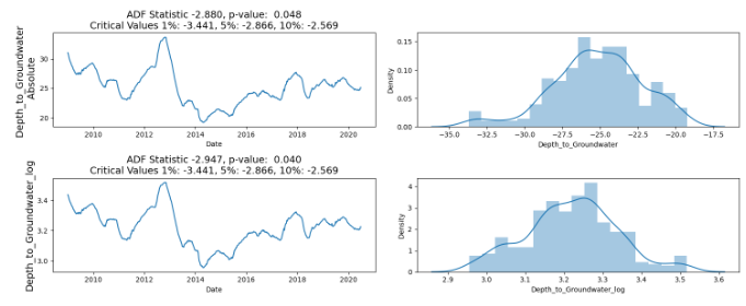

평균과 분산이 좀 더 대칭을 이루며 종 모양과 가까워진 것을 확인할 수 있다. 

 

 

# 1차 차분
ts_diff = np.diff(df.Depth_to_Groundwater)
df['Depth_to_Groundwater_df_1']= np.append([0], ts_diff) #차분으로 삭제된 첫 행 붙여주기

# 2차 차분
ts_diff = np.diff(df.Depth_to_Groundwater_df_1)
df['Depth_to_Groundwater_df_2'] = np.append([0], ts_diff)

# 차분한 데이터 시각화
f, ax = plt.subplots(nrows = 2, ncols = 1, figsize = (15,6))

visualize_adfuller_results(df.Depth_to_Groundwater_df_1, 
                           'Depth_to_Groundwater_df_1', ax[0])
visualize_adfuller_results(df.Depth_to_Groundwater_df_2, 
                           'Depth_to_Groundwater_df_2', ax[1])
plt.tight_layout()
plt.show()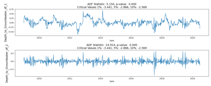

2차 차분한 데이터의 분포가 1차 차분한 데이터보다 일정한 것을 확인할 수 있다.

 

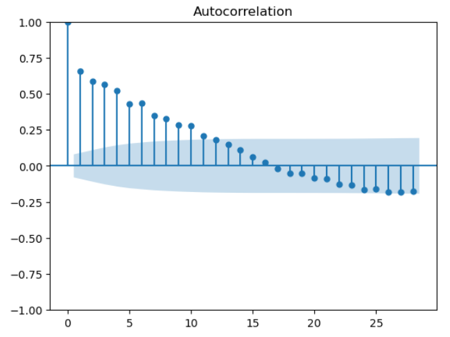
# 2차 차분 acf, pacf 확인

plot_acf(df.Depth_to_Groundwater_df_2)
plt.show()

plot_pacf(df.Depth_to_Groundwater_df_2)
plt.show()

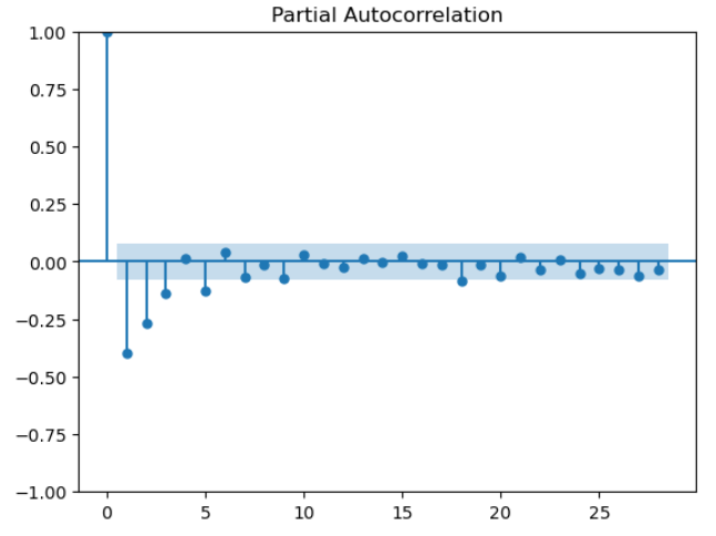
ACF는 시차 2부터 절단면 안에 값이 들어오고 PACF는 시차 4부터 절만면 안에 들어오는 것을 확인할 수 있다.

따라서, p는 3 q는 1로 설정하였다

 

train_df = df[['Date', 'Depth_to_Groundwater_df_2']]
train_df.set_index('Date', inplace = True)

train = train_df.loc['2009-01-01' : '2019-11-28']
test = train_df.loc['2019-12-05':'2020-06-25']

model = ARIMA(train['Depth_to_Groundwater_df_2'], order = (3,2,1))
model_fit = model.fit()
print(model_fit.summary())

AIC가 -507.6이 나왔는데 AIC는 0에 가까울수록 성능이 좋기 때문에 그다지 좋은 결과는 아닌 것 같다

 

# 다음 30개의 데이터 예측
pred = model_fit.forecast(steps = 30)
pred = pd.Series(pred, index = test.index)

fig, ax = plt.subplots(figsize = (15,5))

sns.lineplot(x = 'Date', y = 'Depth_to_Groundwater', data = train)
pred.plot(ax = ax, color = 'red', label = 'Predicted', legend = True)
test.plot(ax = ax, color = 'blue', legend = True)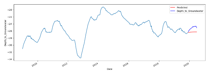

예측 결과를 시각화한 결과, 예상대로 별로 좋지 않다

 

endog_variable = 'Depth_to_Groundwater'
train_y = train[endog_variable]

# 파라미터 최적화
p = range(0,4)
d = range(0,3)
q = range(0,4)
pdq = list(itertools.product(p,d,q))

aic = []
for i in pdq:
    model = ARIMA(train_y, order = i)
    model_fit = model.fit()
    print(f'ARIMA : {i} >> AIC : {round(model_fit.aic, 2)}')
    aic.append(abs(round(model_fit.aic,2)))

optimal = [(pdq[i],j) for i,j in enumerate(aic) if j == min(aic)]
optimal

 

AIC 값이 0에 가장 가까운 p,d,q 조합을 찾는 코드다.

p = 1, d = 0, q = 0의 조합이 AIC 결과가 가장 0에 가깝게 나왔다.

---

 

Ref

https://www.youtube.com/watch?v=abOIK40QvDA&t=640s

https://www.kaggle.com/code/iamleonie/intro-to-time-series-forecasting

https://dacon.io/competitions/official/236200/codeshare/9519 ( 최적의 파라미터 설정 코드 참고)

 

비전공자의 데이터 분석 독학 블로그로

언제든 피드백 환영입니다!